For this challenge we were given a large .pcap file containing some junk traffic and an RTP stream. We extracted the RTP stream using a simple script below. The script expects network capture in .pcapng format as it is even simplier to parse than pcap format.
    import struct

    f = open('ctf-hxp-forensics200.pcapng', 'rb')
    out = open('rtp.raw', 'wb')

    data = f.read(8)
    while len(data) == 8:
        [packetType, packetSize] = struct.unpack("<LL", data)
        data += f.read(packetSize - 8)

        if packetType == 6:
            data = data[0x1C:]  # skip pcap header
            data = data[:-4]  # skip pcap header
            destPort = struct.unpack(">H", data[0x26:0x28])[0] # extract udp dest port
            if destPort == 39194:
                out.write(data[0x38:])

        data = f.read(8)
After the extraction we are ready to import the data into Audacity, as signed 16-bit PCM stereo at 44.1kHz, as was described in RTP headers.
To see the full spectrogram we need to unzoom the frequency range as the spectrogram in Audacity was limited to 8kHz and the information necessary to decode the flag was hidden.
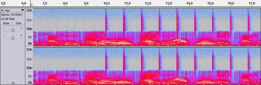
Upon closer inspection, there seem to be a small differences between the spikes starting at 10 seconds. To make them stand out more, I fiddled with spectrogram settings and by increasing the window size and lowering gain, I got them easily recognizable from each other.
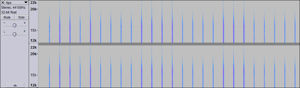
This looks like an binary ascii data, whereas low spikes represent a binary zero and high spikes a binary one. After transcribing them we get: hxp{sry_no_unicorns}
jjk